FIFA World Cup - Qatar 2022

FIFA World Cup - Qatar 2022

At the time of writing the 2022 World Cup is already underway, with 32 teams battling it out in Qatar for the famous golden globe. I’ve lost touch a bit in recent years with football, and thought it would be interesting to use Python to get back up to speed.

The main aim of this project is to try and uncover some insights about the 32 teams - who has played it safe, and gone for experience, who has been bold and decided to give youth a chance to flourish. I’m also interested in where the players play their football at club level, and hope to quantify their geographical spread.

Data source

The data was sourced from Sporting News website.

Exploratory Data Analysis

Let’s dive in!

footbal dive.jpg

## Import the required packages
import pandas as pd
import numpy as np
from pathlib import Path
import matplotlib as plt

pd.options.display.float_format = '{:.2f}'.format

# Load in our data
world_cup = pd.read_csv('Data/World_Cup_2022.csv')

We can automate some of the exploratory data analysis by writing a function:

def initial_eda(df):
    if isinstance(df, pd.DataFrame):
        total_na = df.isna().sum().sum()
        print("Dimensions : %d rows, %d columns" % (df.shape[0], df.shape[1]))
        print("Total NA Values : %d " % (total_na))
        print("%38s %10s     %10s %10s" % ("Column Name", "Data Type", "#Distinct", "NA Values"))
        col_name = df.columns
        dtyp = df.dtypes
        uniq = df.nunique()
        na_val = df.isna().sum()
        for i in range(len(df.columns)):
            print("%38s %10s   %10s %10s" % (col_name[i], dtyp[i], uniq[i], na_val[i]))
        
    else:
        print("Expect a DataFrame but got a %15s" % (type(df)))  

initial_eda(world_cup)

Dimensions : 830 rows, 11 columns
Total NA Values : 0 
                           Column Name  Data Type      #Distinct  NA Values
                                  Name     object          830          0
                              Position     object            4          0
                                   Age    float64           29          0
                               Country     object           32          0
                              Ctry_cap     object           32          0
                                  Caps      int64          132          0
                                 Group     object            8          0
                                  Club     object          446          0
                             Club_ctry     object           43          0
                         Club_ctry_cap     object           43          0
                             Home_Away     object            2          0

Looks like there is no missing data within the dataset. However, there are 8 groups of 4, so 32 teams competing and the maximum permitted squad size is 26, which would be 832 players. We only have 830 observations. Let’s investigate this by grouping the squad numbers by country:

world_cup.groupby("Country")["Name"].count().sort_values(ascending=False)

Country
Argentina       26
Australia       26
Uruguay         26
USA             26
Tunisia         26
Switzerland     26
Spain           26
South Korea     26
Serbia          26
Senegal         26
Saudi Arabia    26
Qatar           26
Portugal        26
Poland          26
Netherlands     26
Morocco         26
Mexico          26
Japan           26
Ghana           26
Germany         26
England         26
Ecuador         26
Denmark         26
Croatia         26
Costa Rica      26
Canada          26
Cameroon        26
Brazil          26
Belgium         26
Wales           26
Iran            25
France          25
Name: Name, dtype: int64

Iran and France only have 25 players in their squad. On follow up this was confirmed to be correct, so we haven’t lost any players! Let’s move on and take a closer look at our data by looking at the first few rows:

# View the first 5 rows
world_cup.head()

	Name	Position	Age	Country	Ctry_cap	Caps	Group	Club	Club_ctry	Club_ctry_cap	Home_Away
0	Saad Al-Sheeb	GK	32.00	Qatar	Doha	80	A	Al-Sadd	Qatar	Doha	Home
1	Meshaal Barsham	GK	24.00	Qatar	Doha	15	A	Al-Sadd	Qatar	Doha	Home
2	Yousuf Hassan	GK	26.00	Qatar	Doha	9	A	Al-Gharafa	Qatar	Doha	Home
3	Pedro Miguel	DEF	32.00	Qatar	Doha	78	A	Al-Sadd	Qatar	Doha	Home
4	Musaab Khidir	DEF	29.00	Qatar	Doha	29	A	Al-Sadd	Qatar	Doha	Home

….and the last few rows:

# View the last 5 rows
world_cup.tail()

	Name	Position	Age	Country	Ctry_cap	Caps	Group	Club	Club_ctry	Club_ctry_cap	Home_Away
825	Kamaldeen Sulemana	MID	20.00	Ghana	Accra	11	H	Stade Rennes	France	Paris	Away
826	Antoine Semenyo	FWD	22.00	Ghana	Accra	1	H	Bristol City	England	London	Away
827	Andre Ayew	FWD	32.00	Ghana	Accra	107	H	Al Sadd	Qatar	Doha	Away
828	Jordan Ayew	FWD	31.00	Ghana	Accra	82	H	Crystal Palace	England	London	Away
829	Inaki Williams	FWD	28.00	Ghana	Accra	1	H	Athletic Club	Spain	Madrid	Away

OK, so we can see that we have some basic information about each player:

- Name
- Position (GK = Goalkeeper DEF = Defender MID = Midfielder FWD = Forward)
- Age
- Country they represent
- Ctry_cap - capital of country they represent
- Caps (Number of matches played for their country)
- Group (32 teams divided into 8 groups A-H of 4)
- Club (the team that pays the player's wages!)
- Club_ctry (the location of the player's domestic team)
- Club_ctry_cap (capital of their club country)
- Home_Away - where they play their club football

Numeric features

import numpy as np

world_cup.describe(include=(np.number))

	Age	Caps
count	830.00	830.00
mean	26.80	33.87
std	4.59	33.81
min	0.00	0.00
25%	24.00	8.00
50%	27.00	23.00
75%	30.00	47.00
max	45.00	191.00

You can’t win anything with kids

It turned out of course that Alan was wrong - Manchester United went on to win the English Premier league that season. There is no master recipe for success it seems at these tournaments. Some managers like to lean on the old guard, some like to throw the gauntlet down and give the kids a chance. Let’s take a look at the age profile of the players using a histogram:

world_cup ['Age'].hist();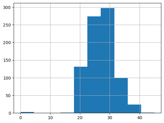

Something doesn’t look right here, some ages between 0 and 5! Let’s look into this. We can use .loc to access a group of rows and columns by name or .iloc to access by index:

world_cup.loc[world_cup['Age'] <5 ]

	Name	Position	Age	Country	Ctry_cap	Caps	Group	Club	Club_ctry	Club_ctry_cap	Home_Away
34	Diego Palacios	DEF	2.00	Ecuador	Quito	11	A	LAFC	USA	Washington, DC	Away
520	Ahmed Reda Tagnaouti	GK	3.00	Morocco	Rabat	3	F	Wydad Casablanca	Morocco	Rabat	Home
642	Fabian Rieder	MID	0.00	Switzerland	Berne	0	G	Young Boys	Switzerland	Berne	Home

On follow up, Diego Palacios Fabian Redier is 23, Ahmed Reda Tagnaouti is 26, and Fabian Rieder is 20 years old. We can correct these errors using .iat. The values we wish to update are located at rows 34, 520 and 642 of column 2 - watch out, indexing starts at 0 in Python!

# Update Diego Palacios age
world_cup.iat[34,2]=23

# Update Ahmed Reda Tagnaouti age
world_cup.iat[520,2]=26

# Update Fabian Rieder age
world_cup.iat[642,2]=20

Let’s check that’s worked:

world_cup.loc[34:34]

	Name	Position	Age	Country	Ctry_cap	Caps	Group	Club	Club_ctry	Club_ctry_cap	Home_Away
34	Diego Palacios	DEF	23.00	Ecuador	Quito	11	A	LAFC	USA	Washington, DC	Away

world_cup.loc[520:520]

	Name	Position	Age	Country	Ctry_cap	Caps	Group	Club	Club_ctry	Club_ctry_cap	Home_Away
520	Ahmed Reda Tagnaouti	GK	26.00	Morocco	Rabat	3	F	Wydad Casablanca	Morocco	Rabat	Home

world_cup.loc[642:642]

	Name	Position	Age	Country	Ctry_cap	Caps	Group	Club	Club_ctry	Club_ctry_cap	Home_Away
642	Fabian Rieder	MID	20.00	Switzerland	Berne	0	G	Young Boys	Switzerland	Berne	Home

Great, the ages have been successfully updated. Let’s now take a look at the age profile of each of the 32 squads:

import matplotlib.pyplot as plt

title_string = "FIFA World Cup - Qatar 2022"
subtitle_string = "Average age of squad"

x = world_cup.groupby('Country')['Age'].mean().sort_values()
plt.figure()
x.plot(kind='barh')
plt.suptitle(title_string, y=1.05, fontsize=18)
plt.title(subtitle_string, fontsize=10)

Text(0.5, 1.0, 'Average age of squad')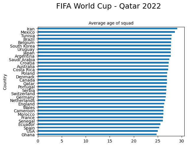

ave_age = world_cup.groupby("Country")["Age"].mean()
ave_age.sort_values(ascending=False)

Country
Iran           29.08
Mexico         28.58
Tunisia        27.92
Brazil         27.86
Belgium        27.77
South Korea    27.77
Uruguay        27.73
Japan          27.69
Argentina      27.69
Saudi Arabia   27.38
Croatia        27.31
Australia      27.23
Costa Rica     27.15
Poland         27.00
Canada         26.92
Denmark        26.92
Qatar          26.92
Portugal       26.77
Serbia         26.77
Switzerland    26.73
Germany        26.69
Netherlands    26.58
England        26.35
Wales          26.23
Morocco        26.19
Cameroon       26.19
France         26.12
Senegal        26.04
Ecuador        25.54
Spain          25.31
USA            25.00
Ghana          24.73
Name: Age, dtype: float64

So Ghana and Ecaudor have the youngest squads (average age 24.73) whilst Iran has the oldest, with an average age of 29.08.

Out with the old

The players below will be looking at the board and hoping for a large number. Players are looking after themselves more and more, extending their playing careers, but realistically, for the players below, this is possibly their last opportunity to appear in a World Cup. So make sure to see catch them while you can!

mature = world_cup[world_cup['Age'] > 33]
mature_sorted = mature.sort_values(by="Age",ascending = False)
mature_sorted.head(10)

	Name	Position	Age	Country	Ctry_cap	Caps	Group	Club	Club_ctry	Club_ctry_cap	Home_Away
143	Ramin Rezaeian	DEF	45.00	Iran	Tehran	2	B	Sepahan	Iran	Tehran	Home
261	Alfredo Talavera	GK	40.00	Mexico	Mexico City	40	C	FC Juarez	Mexico	Mexico City	Home
440	Eiji Kawashima	GK	39.00	Japan	Tokyo	95	E	Strasbourg	France	Paris	Away
781	Pepe	DEF	39.00	Portugal	Lisbon	128	H	Porto	Portugal	Lisbon	Home
608	Atiba Hutchinson	MID	39.00	Canada	Ottawa	98	F	Besiktas	Turkey	Istanbul	Away
682	Dani Alves	DEF	39.00	Brazil	Brasilia	125	G	Pumas UNAM	Mexico	Mexico City	Away
679	Thiago Silva	DEF	38.00	Brazil	Brasilia	108	G	Chelsea	England	London	Away
78	Remko Pasveer	GK	38.00	Netherlands	Amsterdam	2	A	Ajax	Netherlands	Amsterdam	Home
340	Aymen Mathlouthi	GK	38.00	Tunisia	Tunis	73	D	Etoile du Sahel	Tunisia	Tunis	Home
365	Steve Mandanda	GK	37.00	France	Paris	34	D	Rennes	France	Paris	Home

In with the new

new = world_cup[world_cup['Age'] < 20]
new_sorted = new.sort_values(by="Age",ascending = True)
new_sorted.head(10)

	Name	Position	Age	Country	Ctry_cap	Caps	Group	Club	Club_ctry	Club_ctry_cap	Home_Away
435	Youssoufa Moukoko	FWD	17.00	Germany	Berlin	1	E	Borussia Dortmund	Germany	Berlin	Home
820	Fatawu Issahaku	MID	18.00	Ghana	Accra	11	H	Sporting	Portugal	Lisbon	Away
577	Zeno Debast	DEF	18.00	Belgium	Brussels	3	F	Anderlecht	Belgium	Brussels	Home
531	Bilal El Khannouss	MID	18.00	Morocco	Rabat	0	F	Racing Genk	Belgium	Brussels	Away
505	Jewison Bennette	MID	18.00	Costa Rica	San Jose	7	E	Sunderland	England	London	Away
412	Garang Kuol	FWD	18.00	Australia	Canberra	1	D	Central Coast Mariners	Australia	Canberra	Home
478	Gavi	MID	18.00	Spain	Madrid	13	E	Barcelona	Spain	Madrid	Home
784	Antonio Silva	DEF	19.00	Portugal	Lisbon	0	H	Benfica	Portugal	Lisbon	Home
648	Simon Ngapandouetnbu	GK	19.00	Cameroon	Yaounde	0	G	Marseille	France	Paris	Away
504	Brandon Aguilera	MID	19.00	Costa Rica	San Jose	4	E	Guanacasteca	Costa Rica	San Jose	Home

So it looks like the youngest player at the tournament is Youssoufa Moukoko of Germany at just 17.

Are you experienced?

experience.jpg

Although in some sports physical caps may not now always be given (whether at all or for each appearance) the term cap for an international or other appearance has been retained as an indicator of the number of occasions on which a sportsperson has represented a team in a particular sport. Thus, a “cap” is awarded for each game played and so a player who has played x games for the team is said to have been capped x times or have won x caps.

Let’s first look at the distribution of the number of caps received going into this tournament, using a histogram:

world_cup ['Caps'].hist();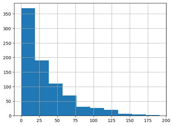

As we can see the majority of players are relatively inexperienced, with less than around 40 appearances, although there are some very experienced players, with over 150 caps. Let’s have a look at who they are:

world_cup.loc[world_cup['Caps'] > 150]

	Name	Position	Age	Country	Ctry_cap	Caps	Group	Club	Club_ctry	Club_ctry_cap	Home_Away
20	Hassan Al-Haydos	MID	31.00	Qatar	Doha	160	A	Al-Sadd	Qatar	Doha	Home
232	Lionel Messi	FWD	35.00	Argentina	Buenos Aires	165	C	PSG	France	Paris	Away
272	Andres Guardado	MID	36.00	Mexico	Mexico City	180	C	Real Betis	Spain	Madrid	Away
506	Celso Borges	MID	34.00	Costa Rica	San Jose	154	E	Alajuelense	Costa Rica	San Jose	Home
558	Luka Modric	MID	37.00	Croatia	Zagreb	155	F	Real Madrid	Spain	Madrid	Away
733	Diego Godin	DEF	36.00	Uruguay	Montevideo	159	G	Velez Sarsfield	Argentina	Buenos Aires	Away
798	Cristiano Ronaldo	FWD	37.00	Portugal	Lisbon	191	H	Manchester United	England	London	Away

Cristiano Ronaldo is the most capped player at the tournament with 191. The 200 mark is in sight, although at 37 maybe it’s time to make way for some new blood?

Baptism of fire?

The minimum number of caps shown is 0 which means there are players at this tournament who have yet to play for their country - the stage has been set! Let’s find out who they are:

world_cup.loc[world_cup['Caps'] == 0]

	Name	Position	Age	Country	Ctry_cap	Caps	Group	Club	Club_ctry	Club_ctry_cap	Home_Away
12	Jassim Jabir	MID	20.00	Qatar	Doha	0	A	Al-Arabi	Qatar	Doha	Home
33	William Pacho	DEF	21.00	Ecuador	Quito	0	A	Royal Antwerp	Belgium	Brussels	Away
50	Kevin Rodriguez	FWD	22.00	Ecuador	Quito	0	A	Imbabura SC	Ecuador	Quito	Home
61	Moussa Ndiaye	DEF	20.00	Senegal	Dakar	0	A	Anderlecht	Belgium	Brussels	Away
70	Pathe Ciss	MID	28.00	Senegal	Dakar	0	A	Rayo Vallecano	Spain	Madrid	Away
79	Andries Noppert	GK	28.00	Netherlands	Amsterdam	0	A	Heerenveen	Netherlands	Amsterdam	Home
83	Jeremie Frimpong	DEF	21.00	Netherlands	Amsterdam	0	A	Bayer Leverkusen	Germany	Berlin	Away
92	Xavi Simons	MID	19.00	Netherlands	Amsterdam	0	A	PSV Eindhoven	Netherlands	Amsterdam	Home
234	Nawaf Al-Aqidi	GK	22.00	Saudi Arabia	Riyadh	0	C	Al-Nassr FC	Saudi Arabia	Riyadh	Home
235	Mohamed Al-Yami	GK	25.00	Saudi Arabia	Riyadh	0	C	Al-Ahli Saudi FC	Saudi Arabia	Riyadh	Home
366	Axel Disasi	DEF	24.00	France	Paris	0	D	Monaco	France	Paris	Home
474	Alejandro Balde	DEF	19.00	Spain	Madrid	0	E	Barcelona	Spain	Madrid	Home
531	Bilal El Khannouss	MID	18.00	Morocco	Rabat	0	F	Racing Genk	Belgium	Brussels	Away
597	James Pantemis	GK	25.00	Canada	Ottawa	0	F	CF Montreal	Canada	Ottawa	Home
624	Philipp Kohn	GK	24.00	Switzerland	Berne	0	G	RB Salzburg	Austria	Vienna	Away
642	Fabian Rieder	MID	20.00	Switzerland	Berne	0	G	Young Boys	Switzerland	Berne	Home
648	Simon Ngapandouetnbu	GK	19.00	Cameroon	Yaounde	0	G	Marseille	France	Paris	Away
779	Jose Sa	GK	29.00	Portugal	Lisbon	0	H	Wolves	England	London	Away
784	Antonio Silva	DEF	19.00	Portugal	Lisbon	0	H	Benfica	Portugal	Lisbon	Home
802	Goncalo Ramos	FWD	21.00	Portugal	Lisbon	0	H	Benfica	Portugal	Lisbon	Home
806	Ibrahim Danlad	GK	19.00	Ghana	Accra	0	H	Asante Kotoko	Ghana	Accra	Home
823	Salis Abdul Samed	MID	22.00	Ghana	Accra	0	H	Lens	France	Paris	Away
824	Kamal Sowah	MID	22.00	Ghana	Accra	0	H	Club Brugge	Belgium	Brussels	Away

As expected, these players are generally quite young (although Portugal’s Jose Sa is 29 - better late than never) or goalkeepers, where the first choice tends to be difficult to oust! Keep an eye out for these names - they might be the stars of the future.

Let’s take a look at the average number of caps for each squad:

import matplotlib.pyplot as plt

title_string = "FIFA World Cup - Qatar 2022"
subtitle_string = "Average number of caps per squad"

x = world_cup.groupby('Country')['Caps'].mean().sort_values()
plt.figure()
x.plot(kind='barh')
plt.suptitle(title_string, y=1.05, fontsize=18)
plt.title(subtitle_string, fontsize=10)

Text(0.5, 1.0, 'Average number of caps per squad')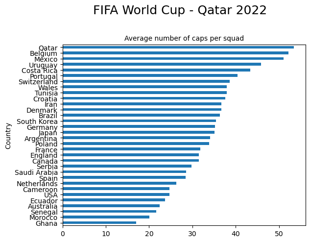

caps = world_cup.groupby("Country")["Caps"].mean()
caps.sort_values(ascending=False)

Country
Qatar          53.46
Belgium        52.19
Mexico         51.12
Uruguay        45.85
Costa Rica     43.42
Portugal       40.42
Switzerland    38.58
Wales          37.96
Tunisia        37.88
Croatia        37.65
Iran           36.72
Denmark        36.65
Brazil         36.31
South Korea    35.46
Germany        35.19
Japan          35.15
Argentina      34.12
Poland         33.88
France         31.80
England        31.54
Canada         31.46
Serbia         29.77
Saudi Arabia   28.50
Spain          28.42
Netherlands    26.23
Cameroon       24.73
USA            24.69
Ecuador        23.73
Australia      22.42
Senegal        21.62
Morocco        20.04
Ghana          17.00
Name: Caps, dtype: float64

The host nation Quatar have the most experienced squad with an average of 53.46 international apperances per player. The least experienced squad is Ghana, with an average of 17.

To caveat this, it is worth noting that qualification for the World Cup is segregated by region, and there can be a wide disparity between the number of qualifying matches played. This can result in some nations playing a large number of matches, without necessarily playing in a major tournament, which is perhaps a better indicator of experience.

Categorical features

Here’s how we get a quick summary of all the non-numeric columns in the dataset:

world_cup.describe(include=[object])

	Name	Position	Country	Ctry_cap	Group	Club	Club_ctry	Club_ctry_cap	Home_Away
count	830	830	830	830	830	830	830	830	830
unique	830	4	32	32	8	446	43	43	2
top	Saad Al-Sheeb	DEF	Qatar	Doha	G	Al-Sadd	England	London	Away
freq	1	274	26	26	130	13	159	159	551

cols = ['Position', 'Group', 'Home_Away']
world_cup[cols] = world_cup[cols].astype('category')

world_cup[['Name','Country','Ctry_cap','Club','Club_ctry','Club_ctry_cap']] = world_cup[['Name','Country','Ctry_cap','Club','Club_ctry','Club_ctry_cap']].astype(str)

Club v Country

First of all let’s look at where these 830 players play their club football:

import matplotlib.pyplot as plt

title_string = "FIFA World Cup - Qatar 2022"
subtitle_string = "Number of players playing in...."

x = world_cup.groupby('Club_ctry')['Club'].count().sort_values(ascending=True).tail(10)
plt.figure()
x.plot(kind='barh')
plt.suptitle(title_string, y=1.05, fontsize=18)
plt.title(subtitle_string, fontsize=16)

Text(0.5, 1.0, 'Number of players playing in....')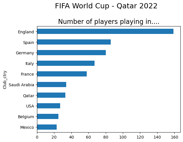

world_cup.groupby("Club_ctry")["Club"].count().sort_values(ascending=False).head(10)

Club_ctry
England         159
Spain            86
Germany          80
Italy            67
France           58
Saudi Arabia     34
Qatar            33
USA              27
Belgium          25
Mexico           23
Name: Club, dtype: int64

So out of 830 players represented at the World Cup, 159 play their football in England. Let’s take a look at the top 10 clubs with the most players playing at this tournament:

title_string = "FIFA World Cup - Qatar 2022"
subtitle_string = "Number of players playing for.."

x = world_cup.groupby("Club")["Club_ctry"].count().sort_values(ascending=True).tail(10)
plt.figure()
x.plot(kind='barh')
plt.suptitle(title_string, y=1.05, fontsize=18)
plt.title(subtitle_string, fontsize=16)

Text(0.5, 1.0, 'Number of players playing for..')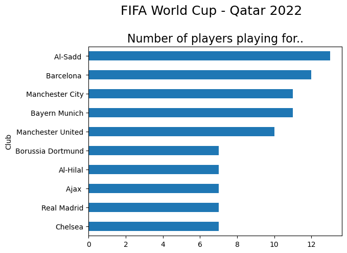

Al-Sadd, wo play in the Qatar Stars league have 13 players (all playing for Qatar) at the tournament, closely followed by Barcelona with 12, Munich and Manchester City, with 11 and Manchester United having 10. Saudi Arabia’s squad all play within Saudi Arabia, 7 of them for Al_Hilal.

Scotland

Sadly, my country didn’t make it, but there are some players who play domestically in Scotland who will be in Qatar representing their country. Let’s have a look and see who they are:

scotland = world_cup[world_cup['Club_ctry'] == 'Scotland']
scotland

	Name	Position	Age	Country	Ctry_cap	Caps	Group	Club	Club_ctry	Club_ctry_cap	Home_Away
159	Cameron Carter-Vickers	DEF	24.00	USA	Washington, DC	10	B	Celtic	Scotland	Edinburgh	Away
200	Dylan Levitt	MID	21.00	Wales	Cardiff	13	B	Dundee United	Scotland	Edinburgh	Away
392	Aziz Behich	DEF	31.00	Australia	Canberra	53	D	Dundee United	Scotland	Edinburgh	Away
394	Nathaniel Atkinson	DEF	23.00	Australia	Canberra	5	D	Hearts	Scotland	Edinburgh	Away
397	Kye Rowles	DEF	24.00	Australia	Canberra	3	D	Hearts	Scotland	Edinburgh	Away
400	Aaron Mooy	MID	32.00	Australia	Canberra	53	D	Celtic	Scotland	Edinburgh	Away
403	Keanu Baccus	MID	29.00	Australia	Canberra	53	D	St Mirren	Scotland	Edinburgh	Away
404	Cameron Devlin	MID	24.00	Australia	Canberra	1	D	Hearts	Scotland	Edinburgh	Away
464	Daizen Maeda	FWD	25.00	Japan	Tokyo	8	E	Celtic	Scotland	Edinburgh	Away
548	Borna Barisic	DEF	29.00	Croatia	Zagreb	28	F	Rangers	Scotland	Edinburgh	Away
554	Josip Juranovic	DEF	27.00	Croatia	Zagreb	21	F	Celtic	Scotland	Edinburgh	Away
614	David Wotherspoon	MID	32.00	Canada	Ottawa	10	F	St. Johnstone	Scotland	Edinburgh	Away

Interestingly, out of the 12 players who play their club football in Scotland, 6 are Australian. The shared language is probably a contributory factor, certainly not the search for warmer weather.

Poland

Having recently relocated here, at least I now have a team to follow! Let’s have a look at the players who play their club football in Poland:

poland_club = world_cup[world_cup['Club_ctry'] == 'Poland']
poland_club

	Name	Position	Age	Country	Ctry_cap	Caps	Group	Club	Club_ctry	Club_ctry_cap	Home_Away
295	Artur Jedrzejczyk	DEF	34.00	Poland	Warsaw	40	C	Legia Warsaw	Poland	Warsaw	Home
297	Michal Skoras	MID	22.00	Poland	Warsaw	1	C	Lech Poznan	Poland	Warsaw	Home
301	Kamil Grosicki	MID	34.00	Poland	Warsaw	87	C	Pogon Szczecin	Poland	Warsaw	Home
706	Filip Mladenovic	DEF	31.00	Serbia	Belgrade	20	G	Legia Warsaw	Poland	Warsaw	Away

Only 4 players, 3 of which are Polish. The lone soldier is Filip Mladenovic of Serbia who plays his club football with Legia Warsaw. Let’s have a look at the Poland squad in general:

poland = world_cup[world_cup['Country'] == 'Poland']
poland

	Name	Position	Age	Country	Ctry_cap	Caps	Group	Club	Club_ctry	Club_ctry_cap	Home_Away
285	Wojciech Szczesny	GK	32.00	Poland	Warsaw	66	C	Juventus	Italy	Rome	Away
286	Lukasz Skorupski	GK	31.00	Poland	Warsaw	8	C	Bologna	Italy	Rome	Away
287	Kamil Grabara	GK	23.00	Poland	Warsaw	1	C	Copenhagen	Denmark	Copenhagen	Away
288	Jan Bednarek	DEF	26.00	Poland	Warsaw	45	C	Aston Villa	England	London	Away
289	Kamil Glik	DEF	34.00	Poland	Warsaw	99	C	Benevento	Italy	Rome	Away
290	Matty Cash	DEF	25.00	Poland	Warsaw	7	C	Aston Villa	England	London	Away
291	Jakub Kiwior	DEF	22.00	Poland	Warsaw	3	C	Spezia	Italy	Rome	Away
292	Robert Gumny	DEF	24.00	Poland	Warsaw	5	C	FC Augsburg	Germany	Berlin	Away
293	Bartosz Bereszynski	DEF	30.00	Poland	Warsaw	46	C	Sampdoria	Italy	Rome	Away
294	Mateusz Wieteska	DEF	25.00	Poland	Warsaw	2	C	Clermont	France	Paris	Away
295	Artur Jedrzejczyk	DEF	34.00	Poland	Warsaw	40	C	Legia Warsaw	Poland	Warsaw	Home
296	Nicola Zalewski	MID	20.00	Poland	Warsaw	7	C	Roma	Italy	Rome	Away
297	Michal Skoras	MID	22.00	Poland	Warsaw	1	C	Lech Poznan	Poland	Warsaw	Home
298	Grzegorz Krychowiak	MID	32.00	Poland	Warsaw	94	C	Al Shabab	Saudi Arabia	Riyadh	Away
299	Piotr Zielinski	MID	28.00	Poland	Warsaw	74	C	Napoli	Italy	Rome	Away
300	Krystian Bielik	MID	24.00	Poland	Warsaw	5	C	Birmingham	England	London	Away
301	Kamil Grosicki	MID	34.00	Poland	Warsaw	87	C	Pogon Szczecin	Poland	Warsaw	Home
302	Przemyslaw Frankowski	MID	27.00	Poland	Warsaw	26	C	Lens	France	Paris	Away
303	Sebastian Szymanski	MID	23.00	Poland	Warsaw	18	C	Feyenoord	Netherlands	Amsterdam	Away
304	Damian Szymanski	MID	27.00	Poland	Warsaw	9	C	AEK Athens	Greece	Athens	Away
305	Szymon Zurkowski	MID	25.00	Poland	Warsaw	7	C	Fiorentina	Italy	Rome	Away
306	Jakub Kaminski	MID	20.00	Poland	Warsaw	4	C	Wolfsburg	Germany	Berlin	Away
307	Krzysztof Piatek	FWD	27.00	Poland	Warsaw	11	C	Salernitana	Italy	Rome	Away
308	Karol Swiderski	FWD	25.00	Poland	Warsaw	18	C	Charlotte	USA	Washington, DC	Away
309	Arkadiusz Milik	FWD	28.00	Poland	Warsaw	64	C	Juventus	Italy	Rome	Away
310	Robert Lewandowski	FWD	34.00	Poland	Warsaw	134	C	Barcelona	Spain	Madrid	Away

Home and Away

home and away.jpg

These days players travel far and wide to ply their trade. I wondered what the impact of that might be on the tightness of a squad, and thought it would be interesting to take a closer look at where players play domestically.

Let’s take a look at the distribution of where the players play their club football:

world_cup['Home_Away'].value_counts()

Away    551
Home    279
Name: Home_Away, dtype: int64

Most players play their club football outside of their home nation. Let’s illustrate that graphically with a bar plot:

home_away_plot = world_cup.groupby(['Home_Away', 'Country']).size().sort_values(ascending=False).reset_index().pivot(columns='Home_Away', index='Country', values=0)
home_away_plot.plot(kind='barh', stacked=True)

<AxesSubplot: ylabel='Country'>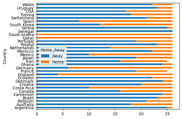

That’s quite insightful and re-emphasises that most players do play their club football outside of their home nation, exemplified at the extreme by Senegal, where the entire squad are based outside of Senegal. At the other extreme, all of the Qatar and Saudi Arabia squads are based at home. England are the next ‘tightest’ squad. Will this contribute to a successful tournament? All will be revealed over the next few weeks!

Huddle

huddle.jpg

We have already established that the total distance for Saudi Arabia and Qatar is zero (their squads all play club football locally), but let’s try to establish just how far flung the other squads are, by calculating the distance for each player from their nation’s capital to the capital of the country where they play their club football.

Apologies for this next section which is not very Pythonic! In hindsight this was probably a tad ambitious for me as someone just starting out, and I ran into all sorts of obstacles, but I got there in the end, and thankfully before the tournament ended!

Obtaining co-ordinates using Geopy

We can obtain the co-ordinates of the capital cities of the countries where the players play their club football using the Geopy library in Python. There is a very useful guide available here:

## Install required package
!pip install geopy

# import required module
from geopy.geocoders import Nominatim

Requirement already satisfied: geopy in /home/stephen137/mambaforge/lib/python3.10/site-packages (2.2.0)
Requirement already satisfied: geographiclib<2,>=1.49 in /home/stephen137/mambaforge/lib/python3.10/site-packages (from geopy) (1.52)

countries = ('England', 'Spain', 'Germany', 'Italy', 'France', 'Saudi Arabia', 'Qatar', 'United States', 'Belgium', 'Mexico', 'Turkey', 'Netherlands', 'Portugal', 'Costa Rica', 'South Korea', 'Greece', 'Scotland', 'Japan',             
'Canada', 'Switzerland', 'Iran',  'Denmark',  'Tunisia',  'Australia',  'Croatia' , 'Brazil',  'Argentina',  'Wales', 'Poland',  'Morocco',  'Ecuador', 'Austria', 'Serbia', 'Uruguay',  'Kuwait', 'Russia',  'Ghana', 'Egypt',                                    
'Cyprus', 'China', 'Cameroon', 'Colombia',  'United Arab Emirates', 'Senegal') 

First, we can create a list of capital cities for the above countries, and then create a function to loop through this list, and extract the longitude and latitude for each of the cities:

# List of capitals
capitals = ['London', 'Madrid', 'Berlin', 'Rome', 'Paris', 'Riyadh', 'Doha', 'Washington, DC', 'Brussels', 'Mexico City', 'Ankara', 'Amsterdam', 'Lisbon', 'San Jose', 'Seoul', 'Athens', 'Edinburgh', 'Tokyo', 
'Ottawa', 'Berne', 'Tehran', 'Copenhagen', 'Tunis', 'Canberra', 'Zagreb', 'Brasilia', 'Buenos Aires', 'Cardiff', 'Warsaw', 'Rabat', 'Quito', 'Vienna', 'Belgrade', 'Montevideo', 'Kuwait City', 'Moscow', 'Accra', 'Cairo',
'Nicosia', 'Beijing', 'Yaounde', 'Bogota','Abu Dhabi','Dakar']

geolocator = Nominatim(user_agent="GetLoc")

# loop through list of capitals and return their co-ordinates
for capital in capitals:
    location = geolocator.geocode(capital)
    lat = location.latitude
    long = location.longitude 
    print(lat,long)

51.5073219 -0.1276474
40.4167047 -3.7035825
52.5170365 13.3888599
41.8933203 12.4829321
48.8588897 2.3200410217200766
24.638916 46.7160104
25.2856329 51.5264162
38.8950368 -77.0365427
50.8465573 4.351697
19.4326296 -99.1331785
39.9207886 32.8540482
52.3727598 4.8936041
38.7077507 -9.1365919
37.3361663 -121.890591
37.5666791 126.9782914
37.9839412 23.7283052
55.9533456 -3.1883749
35.6828387 139.7594549
45.4208777 -75.6901106
46.9482713 7.4514512
35.6892523 51.3896004
55.6867243 12.5700724
33.8439408 9.400138
-35.2975906 149.1012676
45.84264135 15.962231476593626
-10.3333333 -53.2
-34.6075682 -58.4370894
51.4816546 -3.1791934
52.2337172 21.071432235636493
34.022405 -6.834543
-0.2201641 -78.5123274
48.2083537 16.3725042
44.8178131 20.4568974
-34.9058916 -56.1913095
29.3796532 47.9734174
55.7504461 37.6174943
5.5571096 -0.2012376
30.0443879 31.2357257
35.1748976 33.3638568
39.906217 116.3912757
3.8689867 11.5213344
4.6534649 -74.0836453
24.4538352 54.3774014
14.693425 -17.447938

Now create a list which combines the capitals and their co-ordinates:

co_ordinates = [["London", 51.5073219, -0.1276474],
['Madrid', 40.4167047, -3.7035825],
['Berlin', 52.5170365, 13.3888599],
['Rome',  41.8933203, 12.4829321],
['Paris', 48.8588897, 2.3200410217200766],
['Riyadh', 24.638916, 46.7160104],
['Doha', 25.2856329, 51.5264162],
['Washington, DC', 38.8950368, -77.0365427],
['Brussels', 50.8465573, 4.351697],
['Mexico City', 19.4326296, -99.1331785],
['Ankara', 39.9207886, 32.8540482],
['Amsterdam', 52.3727598, 4.8936041],
['Lisbon', 38.7077507, -9.1365919],
['San Jose', 37.3361663, -121.890591],
['Seoul', 37.5666791, 126.9782914],
['Athens', 37.9839412, 23.7283052],
['Edinburgh', 55.9533456, -3.1883749],
['Tokyo', 35.6828387, 139.7594549],
['Ottawa', 45.4208777, -75.6901106],
['Berne', 46.9482713, 7.4514512],
['Tehran', 35.6892523, 51.3896004],
['Copenhagen', 55.6867243, 12.5700724],
['Tunis', 33.8439408, 9.400138],
['Canberra', 35.2975906, 149.1012676],
['Zagreb', 45.84264135, 15.962231476593626],
['Brasilia', -10.3333333, -53.2],
['Buenos Aires', -34.6075682, -58.4370894],
['Cardiff', 51.4816546, -3.1791934],
['Warsaw', 52.2337172, 21.071432235636493],
['Rabat', 34.022405, -6.834543],
['Quito', -0.2201641, -78.5123274],
['Vienna', 48.2083537, 16.3725042],
['Belgrade', 44.8178131, 20.4568974],
['Montevideo', -34.9058916, -56.1913095],
['Kuwait City', 29.3796532, 47.9734174],
['Moscow', 55.7504461, 37.6174943],
['Accra', 5.5571096, -0.2012376],
['Cairo', 30.0443879, 31.2357257],
['Nicosia', 35.1748976, 33.3638568],
['Beijing', 39.906217, 116.3912757],
['Yaounde', 3.8689867, 11.5213344],
['Bogota', 4.6534649, -74.0836453],
['Abu Dhabi', 24.4538352, 54.3774014],
['Dakar', 14.693425, -17.447938]]    

And now create separate DataFrames for our ‘from’ and ‘to’ destinations:

from_co_ord = pd.DataFrame(co_ordinates,columns=['from', 'from_long', 'from_lat'])
to_co_ord = pd.DataFrame(co_ordinates,columns=['to', 'to_long', 'to_lat'])

from_co_ord.head()

	from	from_long	from_lat
0	London	51.51	-0.13
1	Madrid	40.42	-3.70
2	Berlin	52.52	13.39
3	Rome	41.89	12.48
4	Paris	48.86	2.32

to_co_ord.head()

	to	to_long	to_lat
0	London	51.51	-0.13
1	Madrid	40.42	-3.70
2	Berlin	52.52	13.39
3	Rome	41.89	12.48
4	Paris	48.86	2.32

Obtaining all possible city pair combinations

We need to find all the possible ‘from’ : ‘to’ combinations in order to calculate the distances between the cities. We have 44 cities which gives according to this handy calculator , 946 pairings without repetitions.

After some digging around I found this post on stackoverflow which gave a general overview of how this might be achieved. In order to obtain the pairings and index them, we can use the MultiIndex.from_product pandas class:

idx = pd.MultiIndex.from_product([from_co_ord.index, to_co_ord.index], names=['from', 'to'])

# create a combined DataFrame that joins our from and to DataFrames
# Includes all possible pairings (including duplicates)

from_to = pd.DataFrame(index=idx) \
        .join(from_co_ord[['from','from_lat', 'from_long']], on='from') \
        .join(to_co_ord[['to','to_lat', 'to_long']], on='to')

from_to

		from	from_lat	from_long	to	to_lat	to_long
from	to
0	0	London	-0.13	51.51	London	-0.13	51.51
	1	London	-0.13	51.51	Madrid	-3.70	40.42
	2	London	-0.13	51.51	Berlin	13.39	52.52
	3	London	-0.13	51.51	Rome	12.48	41.89
	4	London	-0.13	51.51	Paris	2.32	48.86
...	...	...	...	...	...	...	...
43	39	Dakar	-17.45	14.69	Beijing	116.39	39.91
	40	Dakar	-17.45	14.69	Yaounde	11.52	3.87
	41	Dakar	-17.45	14.69	Bogota	-74.08	4.65
	42	Dakar	-17.45	14.69	Abu Dhabi	54.38	24.45
	43	Dakar	-17.45	14.69	Dakar	-17.45	14.69

1936 rows × 6 columns

That’s not quite as concise as we would like - we have 1936 pairings. That’s because MultiIndex.from_prodcut has returned values for London to London, Dakar to Dakar, etc. We also have London to Madrid, and Madrid to London which is also duplication. Let’s move forward.

Going the extra mile

proclaimers.jpg

We can calculate the distance between two locations using Haversine. Let’s create a function that allows us to return values for all our pairings:

def haversine_np(lon1, lat1, lon2, lat2):
    """
    Calculate the great circle distance between two points
    on the earth (specified in decimal degrees)

    All args must be of equal length.    

    """
    lon1, lat1, lon2, lat2 = map(np.radians, [lon1, lat1, lon2, lat2])

    dlon = lon2 - lon1
    dlat = lat2 - lat1

    a = np.sin(dlat/2.0)**2 + np.cos(lat1) * np.cos(lat2) * np.sin(dlon/2.0)**2

    c = 2 * np.arcsin(np.sqrt(a))
    km = 6367 * c
    miles = km * 0.621371
    return miles

# Add a new column to our from_to DataFrame to include the distance calculations
from_to['Distance_miles'] = haversine_np(*from_to[['from_lat', 'from_long', 'to_lat', 'to_long']].values.T)

Let’s take a look at our completed distances DataFrame:

from_to

		from	from_lat	from_long	to	to_lat	to_long	Distance_miles
from	to
0	0	London	-0.13	51.51	London	-0.13	51.51	0.00
	1	London	-0.13	51.51	Madrid	-3.70	40.42	784.56
	2	London	-0.13	51.51	Berlin	13.39	52.52	577.80
	3	London	-0.13	51.51	Rome	12.48	41.89	890.44
	4	London	-0.13	51.51	Paris	2.32	48.86	212.47
...	...	...	...	...	...	...	...	...
43	39	Dakar	-17.45	14.69	Beijing	116.39	39.91	7634.29
	40	Dakar	-17.45	14.69	Yaounde	11.52	3.87	2107.38
	41	Dakar	-17.45	14.69	Bogota	-74.08	4.65	3906.72
	42	Dakar	-17.45	14.69	Abu Dhabi	54.38	24.45	4673.86
	43	Dakar	-17.45	14.69	Dakar	-17.45	14.69	0.00

1936 rows × 7 columns

V look up in Python

We now want to include the distance figures in our orginal world_cup DataFrame to allow us to calculate the total distance per squad, which will give us some sort of comaprison of the ‘closeness’ of the 32 teams. I am familiar with this feature in Excel but you can do the same thing in Python. Here is a useful article on how to do it.

Let’s first get our DataFrames tee’d up by adding a common column for joining on:

from_to["from_to"] = from_to['from'] + " to " + from_to['to']
from_to

		from	from_lat	from_long	to	to_lat	to_long	Distance_miles	from_to
from	to
0	0	London	-0.13	51.51	London	-0.13	51.51	0.00	London to London
	1	London	-0.13	51.51	Madrid	-3.70	40.42	784.56	London to Madrid
	2	London	-0.13	51.51	Berlin	13.39	52.52	577.80	London to Berlin
	3	London	-0.13	51.51	Rome	12.48	41.89	890.44	London to Rome
	4	London	-0.13	51.51	Paris	2.32	48.86	212.47	London to Paris
...	...	...	...	...	...	...	...	...	...
43	39	Dakar	-17.45	14.69	Beijing	116.39	39.91	7634.29	Dakar to Beijing
	40	Dakar	-17.45	14.69	Yaounde	11.52	3.87	2107.38	Dakar to Yaounde
	41	Dakar	-17.45	14.69	Bogota	-74.08	4.65	3906.72	Dakar to Bogota
	42	Dakar	-17.45	14.69	Abu Dhabi	54.38	24.45	4673.86	Dakar to Abu Dhabi
	43	Dakar	-17.45	14.69	Dakar	-17.45	14.69	0.00	Dakar to Dakar

1936 rows × 8 columns

world_cup["from_to"] = world_cup['Ctry_cap'] + " to " + world_cup['Club_ctry_cap']
world_cup

	Name	Position	Age	Country	Ctry_cap	Caps	Group	Club	Club_ctry	Club_ctry_cap	Home_Away	from_to
0	Saad Al-Sheeb	GK	32.00	Qatar	Doha	80	A	Al-Sadd	Qatar	Doha	Home	Doha to Doha
1	Meshaal Barsham	GK	24.00	Qatar	Doha	15	A	Al-Sadd	Qatar	Doha	Home	Doha to Doha
2	Yousuf Hassan	GK	26.00	Qatar	Doha	9	A	Al-Gharafa	Qatar	Doha	Home	Doha to Doha
3	Pedro Miguel	DEF	32.00	Qatar	Doha	78	A	Al-Sadd	Qatar	Doha	Home	Doha to Doha
4	Musaab Khidir	DEF	29.00	Qatar	Doha	29	A	Al-Sadd	Qatar	Doha	Home	Doha to Doha
...	...	...	...	...	...	...	...	...	...	...	...	...
825	Kamaldeen Sulemana	MID	20.00	Ghana	Accra	11	H	Stade Rennes	France	Paris	Away	Accra to Paris
826	Antoine Semenyo	FWD	22.00	Ghana	Accra	1	H	Bristol City	England	London	Away	Accra to London
827	Andre Ayew	FWD	32.00	Ghana	Accra	107	H	Al Sadd	Qatar	Doha	Away	Accra to Doha
828	Jordan Ayew	FWD	31.00	Ghana	Accra	82	H	Crystal Palace	England	London	Away	Accra to London
829	Inaki Williams	FWD	28.00	Ghana	Accra	1	H	Athletic Club	Spain	Madrid	Away	Accra to Madrid

830 rows × 12 columns

Finally we can join our two DataFrames together which will give us a distance column and value for each player in the tournament:

inner_join = pd.merge(world_cup, from_to, on='from_to',how='inner')

inner_join

	Name	Position	Age	Country	Ctry_cap	Caps	Group	Club	Club_ctry	Club_ctry_cap	Home_Away	from_to	from	from_lat	from_long	to	to_lat	to_long	Distance_miles
0	Saad Al-Sheeb	GK	32.00	Qatar	Doha	80	A	Al-Sadd	Qatar	Doha	Home	Doha to Doha	Doha	51.53	25.29	Doha	51.53	25.29	0.00
1	Meshaal Barsham	GK	24.00	Qatar	Doha	15	A	Al-Sadd	Qatar	Doha	Home	Doha to Doha	Doha	51.53	25.29	Doha	51.53	25.29	0.00
2	Yousuf Hassan	GK	26.00	Qatar	Doha	9	A	Al-Gharafa	Qatar	Doha	Home	Doha to Doha	Doha	51.53	25.29	Doha	51.53	25.29	0.00
3	Pedro Miguel	DEF	32.00	Qatar	Doha	78	A	Al-Sadd	Qatar	Doha	Home	Doha to Doha	Doha	51.53	25.29	Doha	51.53	25.29	0.00
4	Musaab Khidir	DEF	29.00	Qatar	Doha	29	A	Al-Sadd	Qatar	Doha	Home	Doha to Doha	Doha	51.53	25.29	Doha	51.53	25.29	0.00
...	...	...	...	...	...	...	...	...	...	...	...	...	...	...	...	...	...	...	...
805	Mohammed Kudus	MID	22.00	Ghana	Accra	16	H	Ajax	Netherlands	Amsterdam	Away	Accra to Amsterdam	Accra	-0.20	5.56	Amsterdam	4.89	52.37	3245.62
806	Daniel Kofi-Kyereh	MID	26.00	Ghana	Accra	12	H	Freiburg	Germany	Berlin	Away	Accra to Berlin	Accra	-0.20	5.56	Berlin	13.39	52.52	3333.41
807	Fatawu Issahaku	MID	18.00	Ghana	Accra	11	H	Sporting	Portugal	Lisbon	Away	Accra to Lisbon	Accra	-0.20	5.56	Lisbon	-9.14	38.71	2356.37
808	Osman Bukari	MID	23.00	Ghana	Accra	5	H	Red Star Belgrade	Serbia	Belgrade	Away	Accra to Belgrade	Accra	-0.20	5.56	Belgrade	20.46	44.82	2983.47
809	Andre Ayew	FWD	32.00	Ghana	Accra	107	H	Al Sadd	Qatar	Doha	Away	Accra to Doha	Accra	-0.20	5.56	Doha	51.53	25.29	3674.63

810 rows × 19 columns

title_string = "FIFA World Cup - Qatar 2022"
subtitle_string = "Total miles travelled by squad - from their club country capital to their nation capital"

x = inner_join.groupby('Country')['Distance_miles'].sum().sort_values(ascending=False)
plt.figure()
x.plot(kind='barh')
plt.suptitle(title_string, y=1.05, fontsize=18)
plt.title(subtitle_string, fontsize=10)

Text(0.5, 1.0, 'Total miles travelled by squad - from their club country capital to their nation capital')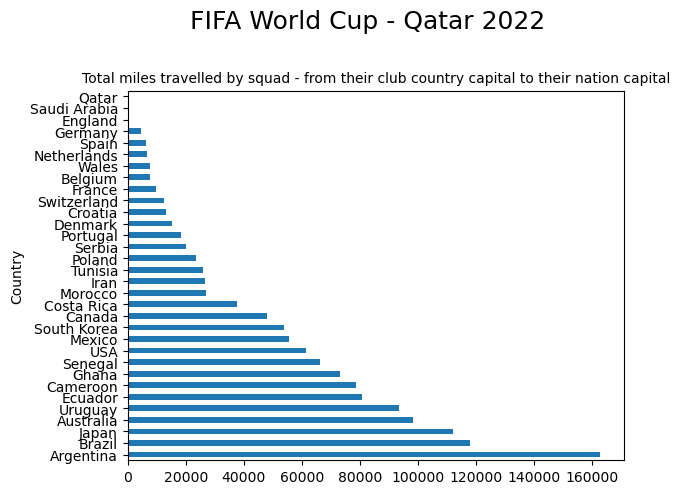

inner_join.groupby("Country")["Distance_miles"].sum().sort_values(ascending=True)

Country
Saudi Arabia        0.00
Qatar               0.00
England           577.80
Germany          4631.29
Spain            6389.33
Netherlands      6658.89
Wales            7674.01
Belgium          7824.11
France           9663.44
Switzerland     12648.83
Croatia         13322.72
Denmark         15194.21
Portugal        18366.13
Serbia          19948.33
Poland          23557.92
Tunisia         25922.17
Iran            26752.28
Morocco         27042.30
Costa Rica      37651.80
Canada          47922.17
South Korea     53858.03
Mexico          55687.73
USA             61448.54
Senegal         66198.44
Ghana           73052.50
Cameroon        78656.09
Ecuador         80700.85
Uruguay         93702.58
Australia       98441.33
Japan          112062.53
Brazil         118045.02
Argentina      162925.56
Name: Distance_miles, dtype: float64

Full time

Home advantage often counts. If you recall South Korea reached the semi final when they hosted the tournament back in 2002, and if you look back even further to 1966 then… Let’s end that there.

Will this togetherness give Qatar an advantage? Time will tell. They also have the ‘tightest’ squad (along with Saudi Arabia) in terms of the fact that all of their players play their club football at home. Outside of those two, England are the ‘closest’ squad, with only Jude Bellingham (Borussia Dortmund) playing his club football outside of England.

The Argentina squad are the most scattered, followed by Brazil, Argentina, and Japan. This makes sense, as most of their squads play in Europe, which is a long way from home!

Key take-aways

This has been a rewarding project overall for me. I achieved what I set out to do, which began with a vague idea of the ‘tightness’ of the World Cup squads, and how I might quantify this, perhaps by looking at where the players play their club football, and how far they would have to travel to begin preparations back in their home nation.

There were many obstacles along the way, the main one was working out how to calculate the distance between two points, and this gave me a first introduction to working with geospatial data, including the Geopy library and Haversine. I also managed to create one or two functions to automate the extraction of co-ordinate data and distance calculations and found about one of the more advanced panda classes, MultiIndex.from_product.

I was familiar with the VLOOKUP fuction in Excel, and the various join clauses in SQL, but I now know how to achieve the same end result using pandas merge.

I’m looking forward to seeing how this Tournament unfolds - may the best team win!